
Office Button: The Office Button is located at the upper-left menu appears. You can use this menu to create a new life, open an existing file, save a file, and perform many other tasks.
Quick Access Toolbar: Quick Access Toolbar is present next of the Office Button. It provides access to commands used frequently. By default, Save, Undo, and Redo appear on the Quick Access Toolbar.
Title bar: The title bar is located at the top. It displays the name of the workbook (a collection of worksheets) on which you are currently working. The right side of the title bar contains Minimize, Restore or Maximize, and Close buttons.
Ribbon: The ribbon is located near the top of the Excel window, below the Quick Access Toolbar. At the top of the ribbon, there are several tabs. Clicking a tab displays related command groups. Within each group, there are related command buttons.
Scroll bar: There are two scroll bars – vertical scroll bar (present on the right) and horizontal scroll bar (present at the bottom).
Status bar: The status bar is present at the bottom of the window and displays status information. The right side of the status bar shows different views like Normal view, Page Layout view, Page Break Preview, and Zoom slider.
Worksheet tabs: A workbook, By default, opens three worksheets named as sheet1, Sheet2, and Sheet3. You can click the sheet tab of a worksheet to open it. To insert more sheets, click Insert Worksheet button.
Cell: A cell is the smallest unit of a worksheet, formed by the intersection of a row and column. Each cell has a unique address formed by the combination of a column and a row number. For example, where row 4 is intersected by the column D, the cell so formed has the address D4.
Name Box: Name box is present on the left side of the formula bar. It gives the address of the selected cell.
Formula Bar: Formula bar displays the constant data or formula used in the active cell. The formula bar is also used for editing the cell contents.
Operators specify the type of calculation that you want to perform on the elements of a formula. Microsoft Excel includes four different types of calculation operators: arithmetic, comparison, text, and reference.
Arithmetic operators: To perform basic mathematical operations such as addition, subtraction, or multiplication; combine numbers; and produce numeric results, use the following arithmetic operators.

Comparison operators: You can compare two values with the following operators. When two values are compared by using these operators, the result is a logical value either TRUE or FALSE.

Text Operator (&): This operator Joins 2 or more text values to produce a single combined text value this operation is known as “Concatenation”.
Example:
- If cell C! contains the text “Total Sales Amount” the formula is = “5% Discount on” & C1, It produces the text value as:
“5% Discount on Total Sale Amount” - If cell A1 contains the text “COMPUTER”
If cell A2 contains the text “APPLICATION”
The formula is =A1&A2 it produces the “COMPUTER APPLICATION”.
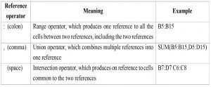
Reference operators: Combine ranges of cells for calculations with the following operators.
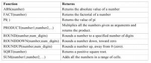
Functions are predefined formulas that perform calculations by using specific values, called arguments, in a particular order, or structure. Functions can be used to perform simple or complex calculations. All function Name begin with a ‘=’ sign
Excel Function can be Categories as follows:-- Mathematical function
- Statistical function
- Date & Time function
- Logical function
1. Mathematical function: These functions are used to calculate the general Calculation. Matrix and trigonometric logarithmic Values etc.
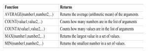
 2. Statistical function:
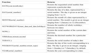
 3. Date & Time function:
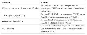
 4. Logical function: Logical functions are used to check the condition if condition is true it performs the test.
NEW BLANK WORKBOOK
- Click Microsoft Office Button , and then click New.
(Keyboard shortcut You can also press CTRL+N.)
SAVE A WORKBOOK
- Click the Microsoft Office Button , and then click Save As.
- In the File name box, enter a new name for the file.
- Click Save.
OPEN A FILE
- Click the Microsoft Office Button , and then click Open.
- On the File menu, click Open.
- Select the cell or the range of cells where you want to insert the new blank cells. Select the same number of cells as you want to insert. For example, to insert five blank cells, you need to select five cells.
- On the Home tab, in the Cells group, click the arrow next to Insert, and then click Insert Cells.
- To insert a single row, select the row or a cell in the row above which you want to insert the new row.
- On the Home tab, in the Cells group, click the arrow next to Insert, and then click Insert Sheet Rows
- To insert a single column, select the column or a cell in the column immediately to the right of where you want to insert the new column
- On the Home tab, in the Cells group, click the arrow next to Insert, and then click Insert Sheet Columns.
- Select the cells, rows, or columns that you want to delete.
- On the Home tab, in the Cells group, do one of the following:
- To delete selected cells, click the arrow next to Delete, and then click Delete Cells.
- To delete selected rows, click the arrow next to Delete, and then click Delete Sheet
- To delete selected columns, click the arrow next to Delete, and then click Delete Sheet Columns.
- To insert a new worksheet before an existing worksheet, select that worksheet, and then on the Home tab, in the Cells group, click Insert, and then click Insert Sheet.
- On the Sheet tab bar, right-click the sheet tab that you want to rename, and then click Rename
- On the Home tab, in the Cells group, click the arrow next to Delete, and then click Delete Sheet
- On the Sheet tab bar, right-click the sheet tab that you want to color, and then click Tab Color, and Choose Color
Set a column to a specific width
- Select the column or columns that you want to change.
- On the Home tab, in the Cells group, click Format.
- Under Cell Size, click Column Width.
- In the Column width box, type the value that you want.
Change the column width to fit the contents
- Select the column or columns that you want to change.
- On the Home tab, in the Cells group, click Format
- Under Cell Size, click AutoFit Column Width
Change the default width for all columns on a worksheet or workbook
- On the Home tab, in the Cells group, click Format
- Under Cell Size, click Default Width.
- In the Default column width box, type a new measurement
Set a row to a specific height
- Select the row or rows that you want to change.
- On the Home tab, in the Cells group, click Format.
- Under Cell Size, click Row Height.
- In the Row height box, type the value that you want.
Change the row height to fit the contents
- Select the row or rows that you want to change.
- On the Home tab, in the Cells group, click Format
- Under Cell Size, click AutoFit Row Height.
Hide a row or column
- Select the rows or columns that you want to hide.
- On the Home tab, in the Cells group, click Format
- Do one of the following:
- Under Visibility, point to Hide & Unhide, and then click Hide Rows or Hide Columns.
- Under Cell Size, click Row Height or Column Width, and then type 0 in the Row Height or Column Width
Display a hidden row or column
To display hidden rows, select the row above and below the rows that you want to display
On the Home tab, in the Cells group, click Format
Do one of the following:
- Under Visibility, point to Hide & Unhide, and then click Unhide Rows or Unhide Columns.
- Under Cell Size, click Row Height or Column Width, and then type the value that you want in the Row Height or Column Width box.
- Select the cell, range of cells, text, or characters that you want to format.
- On the Home tab, in the Font group, do the following:
-
- To change the font, click the font that you want in the Font box Calibri
- To change the font size, click the font size that you want in the Font Size box 12 , or click Increase Font Size Big A icon or Decrease Font Size Small A Icon until the size you want is displayed in the Font Size box.
- Select the cell, range of cells, text, or characters that you want to format.
- On the Home tab, in the Font group, do one of the following:
- To make text bold, click Bold B.
Keyboard shortcut You can also press CTRL+B or CTRL+2. - To make text italic, click Italic I.
Keyboard shortcut You can also press CTRL+I or CTRL+3. - To underline text, click Underline U.
Keyboard shortcut You can also press CTRL+U or CTRL+4.
- On a worksheet, select the cell or range of cells that you want to add a border to, to change the border style on, or to remove a border from
- On the Home tab, in the Font group, do one of the following:
- To apply a new or different border style, click the arrow next to Borders , and then click a border style.
- To remove cell borders, click the arrow next to Borders , and then click No Border .
Fill Cells with Solid colors
- Select the cells that you want to apply shading.
- On the Home tab, in the Font group, do one of the following:
- To fill cells with a solid color, click the arrow next to Fill Color in the Font group on the Home tab, and then click the color on the palette that you want.
- To apply the most recently selected color, click Fill Color
Remove cell shading
- Select the cells that contain a fill color or fill pattern.
- On the Home tab, in the Font group, click the arrow next to Fill Color, and then click No Fill
Alignment refers to the position at which data is placed within the boundary of a cell.
Select the cell that you want to Align.
On the Home tab, in the Alignment group
Click Align Text Left button to left align text
Click Center button to center align text
Click Align Text Right button to right align text
Click Top Align button to Align text to the top off cell
Click Middle Align button to align text so that it is centered between the top and bottom of the cell
Click Bottom Align button to align text to the bottom of the cell
Now select the cell, Click on Orientation, and Click the required option.
Example:
Angle Counterclockwise
Angle Clockwise
Vertical Text
Rotate Text Up
Rotate Text Down
Format Cell Alignment
If you want text to appear on multiple lines in a cell, you can format the cell so that the text wraps automatically, or you can enter a manual line break.
- In a worksheet, select the cells that you want to format.
- On the Home tab, in the Alignment group, click Wrap Text .
Select two or more adjacent cells that you want to merge.
On the Home tab, in the Alignment group, click Merge and Center.
Using the fill handle, you can quickly fill cells in a range with a series of numbers or dates or with a built-in series for days, weekdays, months, or years.
- Select the first cell in the range that you want to fill.
- Type the starting value for the series.
- Type a value in the next cell to establish a pattern.
For example, if you want the series 1, 2, 3, 4, 5…, type 1 and 2 in the first two cells. If you want the series 2, 4, 6, 8…, type 2 and 4. If you want the series 2, 2, 2, 2…, you can leave the second cell blank.
More examples of series that you can fill- Select the cell or cells that contain the starting values.
- Drag the fill handle across the range that you want to fill.
When a date or time is typed in a cell, it appears in a default date and time format. The default date and time format is based on the regional date and time settings that are specified in Windows Control Panel, and changes when changes are made to those settings. You can display numbers in several other date and time formats, most of which are not affected by Control Panel settings.
- Select the cells that you want to format
- On the Home tab, click the Dialog Box Launcher next to Number.
- In the Category list, click Date or Time.
- In the Type list, click the date or time format that you want to use.
Creating a chart in Microsoft Office Excel is quick and easy. Excel provides a variety of chart types that you can choose from when you create a chart.
For most charts, such as column and bar charts, you can plot the data that you arrange in rows or columns on a worksheet in a chart. Some chart types, however, such as pie and bubble charts, require a specific data arrangement.
- On the worksheet, arrange the data that you want to plot in a chart.
- Select the cells that contain the data that you want to use for the chart
- On the Insert tab, in the Charts group, do one of the following:
- Click the chart type, and then click a chart sub-type that you want
- To see all available chart types, click a chart type, and then click All Chart Types to display the Insert Chart dialog box, click the arrows to scroll through all available chart types and chart sub-types, and then click the ones that you want to use.